

In a previous blog post we detailed how we used OCaml to reproduce some classical deep-learning results that would usually be implemented in Python. Here we will do the same with some Reinforcement Learning (RL) experiments.
The previous post was using TensorFlow but this time we will be using PyTorch through some ocaml-torch bindings. This will let us train an agent playing Pong. The PyTorch website features a dedicated reinforcement learning tutorial using the Python api, this tutorial provides more details on RL and on the DQN algorithm that we are using in this post so this is a nice complementary read.
The RL techniques we used here have been explored for a couple of years. The only difference is that we are implementing them in OCaml. Of course, this is fun, but there is a practical benefit too. RL usually involves more infrastructure and code than supervised learning so it’s a place where having a strong type system could be useful, e.g. to let you easily refactor some components without being scared of breaking all the agents that rely on it. Using Python with some good test coverage is the common way to achieve this but with OCaml you can get even stronger guarantees by relying both on testing and on the type system.
Reinforcement Learning
Reinforcement Learning is a sub-field of machine learning where an agent gets to interact with an environment by observing the state of the world, deciding on an action and submitting it to the environment. The environment then updates its state according to this action and returns some new observation as well as a potential reward. The goal for the agent is to maximize the rewards that it gets by interacting with the environment.
Deep Reinforcement Learning combines the modern Deep Learning approach to Reinforcement Learning. One of the early algorithms in this domain is Deepmind’s Deep Q-Learning algorithm which was used to master a wide range of Atari 2600 games. In this context the observations are the values taken by the pixels from the screen (with a resolution of 160x192); the actions correspond to pressing the different buttons, e.g. left, right, or fire, and the rewards come from the score of the game.
In order to interact with Atari games we rely on the OpenAI gym environment, which makes it very easy to try different Atari games or various other tasks. The OCaml signature for the environment is as simple as one would expect:
module Env : sig
  type t

  (** [create ()] sets up a new environment. *)
  val create : unit -> t

  (** [reset t] creates a new game session and returns the first observation. *)
  val reset : t -> observation

  (** [step t ~action] applies [action] to the environment and returns the
      new observation, the reward received by the agent, and a boolean
      set to true if the game has finished. *)
  val step : t -> action:int -> observation * float * bool
end
Q-values
Consider the function which, given a state and an action , returns the total reward that an agent playing perfectly would get starting from state if it used action . If could be computed exactly it would be straightforward to build a perfect agent by selecting the action that maximizes . Most of the time, this function is not known; in a nutshell, Q-learning is the process of approximating it. Deep Q-Networks (DQN) build such an approximation using (deep) neural networks.
We know that must satisfy the Bellman equation which states that is the sum of the reward received when performing action and the Q-value from the next state (as returned by the environment) using the action leading to the highest value.
is the discount factor, a constant between 0 and 1 representing that future rewards are to be discounted, i.e. getting a reward now is better than later. A typical value is .
More generally, any agent defined by a function which maps each state to the action performed on this state has an associated Q-value function that satisfies a similar equation:
Our agent uses the action that maximizes its internal approximation of . So to find a good Q-value approximation we look for a function that approximately satisfies the same Bellman equation as . In particular, we will use a learning algorithm that attempts to minimise the loss
As our Q-value approximation improves, the policy that it implies for the agent accumulates more rewards.
Each optimization step runs the following ocaml-torch snippet, the model we use is called q_model. As we consider that our agent takes the optimal action we take the maximum of the expected values for the next step.
let qvalues = Layer.apply q_model state in
let next_qvalues = Layer.apply q_model next_state |> Tensor.max in
let expected_qvalues = Tensor.(rewards + f gamma * next_qvalues) in
(* minimize the mean squared error between [qvalues] and [expected_qvalues] *)
let loss = Tensor.mse_loss qvalues expected_qvalues in
Optimizer.backward_step t.optimizer ~loss;
When it comes to action selection we use an -greedy policy. Rather than always taking the best action according to the current function there is some small probability at each step of taking a random action instead. This helps the agent discovering new states and so gives more weight to exploration in the exploration vs exploitation tradeoff. The value of decays over time. This corresponds to the following code snippet:
let action t state ~total_frames =
  let epsilon = Float.max 0.02 (0.5 -. Float.of_int total_frames /. 1_000_000.) in
  if Float.(<) epsilon (Random.float 1.)
  then begin
    let qvalues = Layer.apply q_model in
    Tensor.argmax qvalues |> Tensor.to_int0_exn
  end else Random.int t.actions
Modeling Q-values
An observation returned by our environment consists of the pixel values for the whole screen. The color information is not very relevant in Pong so we convert the frame to grayscale and downscale it to 80x80. Seeing a single frame is not enough to know about the ball direction so we consider the difference between two consecutive frames. This is implemented in a pre-processing function with the following signature:
val preprocess : Tensor.t -> Tensor.t
As Andrej Karpathy noted in his blog post Pong from Pixels, there is no need to use convolutions. A simple two layer model is enough do the trick. The input to the model is an 80x80 image that we flatten before applying the first linear layer.
let model vs actions =
  let linear1 = Layer.linear vs ~input_dim:(80 * 80) 200 in
  let linear2 = Layer.linear vs ~input_dim:200 actions in
  Layer.of_fn (fun xs ->
    Tensor.flatten xs
    |> Layer.apply linear1
    |> Tensor.relu
    |> Layer.apply linear2)
An issue with Q-learning is that the states that the agent observes in two consecutive frames are very correlated. Learning only on the most recent data could easily get the agent to ‘forget’ about the more distant past. To mitigate this we use a replay memory to store a large amount of previous transitions. Each transition is composed of a state, an action, the returned reward and the subsequent state. On a training step we extract a random batch of transitions from this memory and hence hopefully provide less correlated data. This process is called experience replay.
The replay memory is implemented by a ring buffer and has the following
signature. The main functions are create, push to add a transition to the
memory and sample to get a random batch of elements from the current memory.
module Replay_memory : sig
  type t
  val create : capacity:int -> t
  val push : t -> transition -> unit
  val sample : t -> batch_size:int -> transition list
end
The training loop then processes one game (or episode) at a time. For each of these an internal loop runs until the game is over by:
- Getting the agent action using the -greedy policy described previously.
- Giving the action to the environment, and getting back the reward and next observation.
- Pushing this transition to the replay memory.
- Extracting a random batch from the replay memory and using it to optimize the approximated function.
This leads to the following OCaml code:
for episode_idx = 1 to total_episodes do
  let rec loop state =
    let action = DqnAgent.action agent state in
    let next_state, reward, is_done = Env.step env ~action in
    let next_state = preprocess next_state in
    (* Add the transition to the replay memory. *)
    Replay_memory.push memory { state; action; next_state; reward; is_done };
    (* Perform an optimization step using a random batch from the replay memory. *)
    let batch = Replay_memory.sample memory ~batch_size in
    DqnAgent.learning_step agent batch;
    if not is_done then loop next_state
  in
  loop (Env.reset env |> preprocess)
done
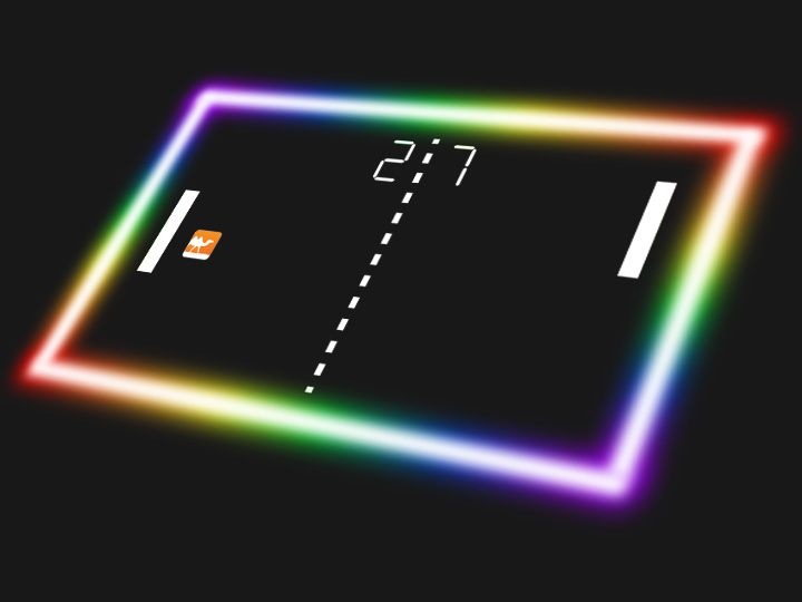
Mastering Pong
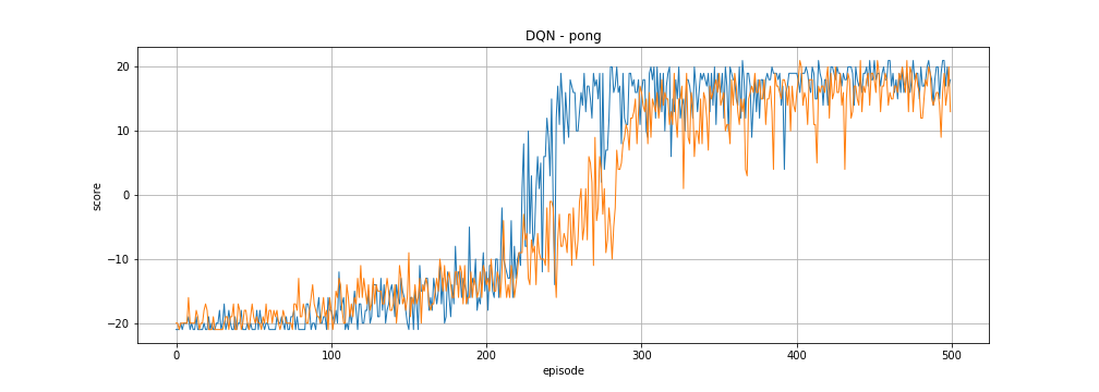
In Pong the player has to bounce a ball back at its opponent. If it misses the opponent gets a point, if the opponent misses the player gets a point. These two events respectively corresponds to a reward of -1 and +1. Each match consists of 21 points. We sum the rewards that the agent receives to get a score that can range from -21 to 21.
The following two curves show the evolution of the scores achieved by our DQN agent in two different training sessions, showing how noisy training is. In both cases it takes a bit more than 100 matches for the agent to manage to score consistently but after that it quickly improves and gets far better than the game hard-coded agent.
We can also visualize the agent playing a match.
The source code for the pong example can be found in the GitHub ocaml-torch repo.
The actual implementation is a bit more involved than what has been described so far. Rather than using a single model for our approximated function , we use an additional target model . The right hand side of the Bellman equation uses and we only update after some fixed number of updates by copying the weights from whereas gets continuously updated. This target Q-network trick is also used in the original DQN paper.
Playing Breakout
Let’s try a more challenging Atari game: Breakout. In order to get DQN to work on this we used the following tweaks.
- The agent’s inputs are still downsampled grayscale images - however this time the agent is given the last 4 frames so that it can infer the movement.
- The model uses a Convolutional Neural Network.
- We use episodic life: each time it loses a life the agent is told that the game is over. This helps the agent more quickly figure out how bad it is to lose a life.
- Rather than the mean square error for the Bellman equation based loss, we use the more robust Huber loss. This has the same effect as clipping the gradients of the loss with respect to the model to 1.
The resulting algorithm takes far longer to train on this game. The following plot shows the training score evolution as a function of the number of frames that have been played (an episode lasts for ~150 to ~2000 frames). Training is very noisy, so the curve shows the score averaged over the last 100 episodes.
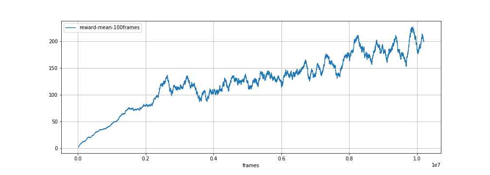
After training for 10 million frames the DQN agent almost manages to clear the screen on its best runs:
The source code can again be found on GitHub.
Improving Type Safety
Using OCaml to implement DQN is a nice exercise, now let’s see what benefits the OCaml type system could bring. For Pong we used a pre-processing function that converts a tensor containing an RGB image of the screen to a lower resolution tensor containing the difference between two consecutive grayscale frames. We also used a two layer model that takes a pre-processed image and returns the Q-values. These functions have the following signatures:
val preprocess : Tensor.t -> Tensor.t
val model : Tensor.t -> Tensor.t
These signatures don’t provide much safety: the number of dimensions for the tensors is not even specified. The following snippet would compile without any type error despite the pre-processing step being omitted. Hopefully a dimension mismatch could help us catch this at runtime but we would rather enforce this in a static way.
let obs, reward, is_done = Env.step env ~action in
(* No pre-processing has been applied! *)
let q_values = model obs in
There have been some interesting discussions recently on how to avoid
this kind of issue, e.g. using Tensor with named
dimensions. Here we
will take a less generic approach. We introduce new types that
abstract the Tensor.t type, have some specified number of
dimensions and also provide more information on what the dimension
represents. We also introduce a couple of empty types to represent the
various dimension types.
type _ tensor1
type (_, _) tensor2
type (_, _, _) tensor3
type (_, _, _, _) tensor4

type n (* batch dimension *)
type c (* channel dimension for images *)
type h (* height dimension for images *)
type w (* width dimension for images *)
type a (* action dimension - for q-values *)
The new types can then be used to reflect the dimensions that we expect for the pre-processing and model functions.
val preprocess : (n, c, h, w) tensor4 -> (n, h, w) tensor3
val model : (n, h, w) tensor3 -> (n, a) tensor2
Now the code snippet where we forgot the pre-processing would not compile anymore. We can also give proper types to some generic functions, e.g. require that the dimensions are the same for a sum or remove the last dimension when taking the maximum over this last dimension.
val add3 : ('a, 'b, 'c) tensor3 -> ('a, 'b, 'c) tensor3 -> ('a, 'b, 'c) tensor3
val max_over_last_dim3 : ('a, 'b, 'c) tensor3 -> ('a, 'b) tensor2
Our encoding was a bit crude so we had to create specific functions depending on the number of dimensions. In the future, this is the kind of thing that modular implicits will help with.